Posterior predictives for AR(p) models in Stan
Autoregressive (AR) models represent a popular type of statistical model. They are used to describe processes which evolve through time. Often then, a statistician is interested in fitting such a model to real data, with the intention of using the fitted model to make predictions about the future.
If you’ve happened upon this post in all likelihood you’re probably already familiar with autoregressive models and Stan. In this case you can skip straight onto the Stan code in the posterior predictives section . Otherwise, read on through and I’ll provide a quick primer on AR models and posterior predictives.
All of the code used in this blog post to simulate the AR model, perform the parameter inference and visualise the output is contained in this github repo
Autoregressive models
An autoregressive model of order \(p\), denoted \(AR(p)\), can be expressed by the relation: \[ X_t = \alpha + \sum_{i=1}^p \beta_i X_{t-i} + \epsilon_t, \] where \(\epsilon_t\) represents random noise. With this, each observation \(X_t\) is related to the \(p\) observations which come before it. The parameters \(\beta_1,\ldots,\beta_p\) determine how \(X_t\) relates to these previous observations.
Presented with observations \((x_1,\ldots,x_n)^T\) the statistician is then tasked with determining values of \(\alpha\) and \(\beta\) which best describe the data. Of course \(p\), the order of the model, must also be determined. A crude method to estimate \(p\) is to assess autocorrelation plots. The order of the model can be estimated as the lag at which the autocorrelation drops below some threshold value.
Simulation studies
A simulation study can be a good way to verify the validity of parameter inference for a given model. The idea is to simulate a model forward for known parameter values. Then, using the data generated from this forward simulation, we attempt to recover the correct parameter values back from the data.
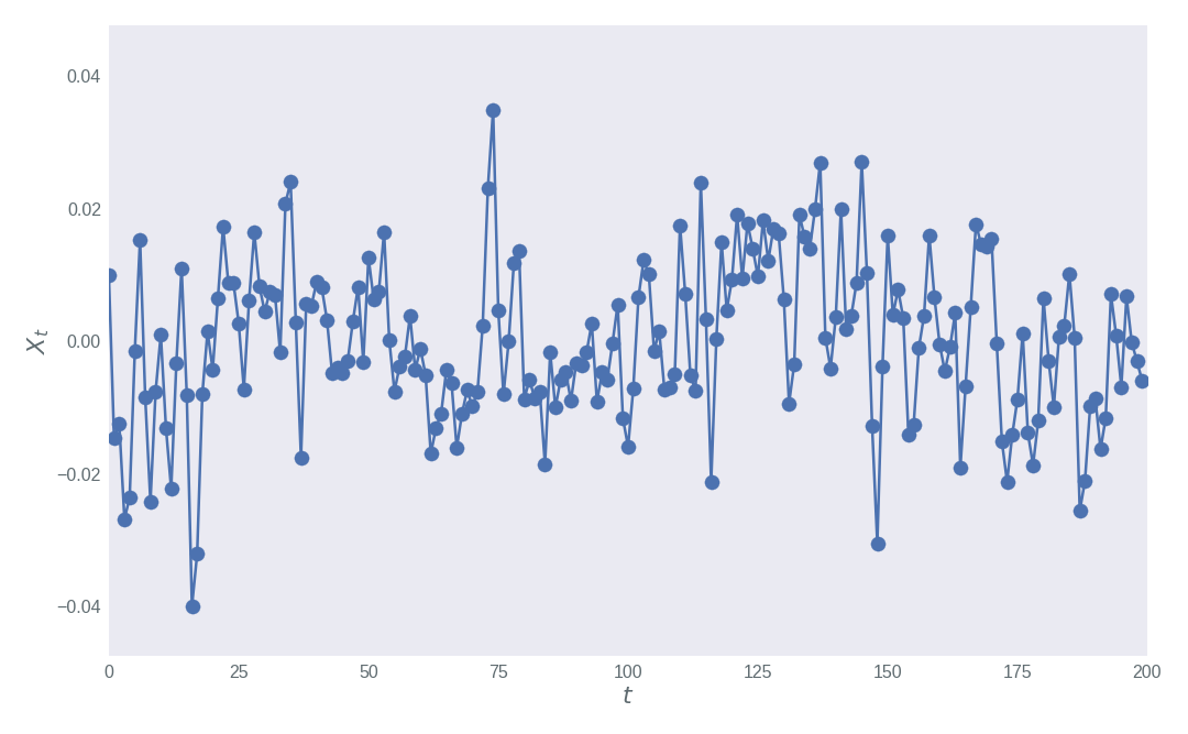
Here I shall forward simulate an \(AR(3)\) model with \(\alpha=0\), \(\beta=(0.75, -0.5,0.25)^T\) and \(\epsilon_t \sim \mathcal{N}(0, 0.01)\). The plot below shows 200 data points realised with these parameter values. The game now is to use the data represented in the plot to infer the values of \(\alpha\), \(\beta\) and the standard deviation of the distribution of \(\epsilon_t\).
Fitting \(AR(p)\) models in Stan
Stan, named after Stanislaw Ulam, is a probabilistic programming language wrote in C++. Stan can be used to perform parameter in a Bayesian framework. The job of the user is to specify how to target a given model’s log-posterior density using Stan’s modelling language.
With the model specified Stan implements the No-U-Turn-Sampler (NUTS), a variant of Hamiltonian Monte Carlo, to draw samples from the posterior distribution. Stan code to infer the parameters \(\alpha\) and \(\beta\) of an \(AR(p)\) model with normally distributed noise can be realised as:
data {
    // Order of AR process
    int<lower=0> P;
    // Numer of observations
    int<lower=0> N;
    // Observations
    vector[N] y;
}
parameters {
    // Additive constant
    real alpha;
    // Coefficients
    vector[P] beta;
    // Standard deviation of the noise
    real<lower=0> sigma;
}
transformed parameters {
    // Consider mu as a transform of the data, alpha and beta
    vector[N] mu;

    // Initial values
    mu[1:P] = y[1:P];

    for (t in (P + 1):N) {
        mu[t] = alpha;
        for (p in 1:P) {
            mu[t] += beta[p] * y[t-p];
        }
    }
}
model {
    // Increment the log-posterior
    y ~ normal(mu, sigma);
}
The nice thing about the above model specification is that it does not hard-code the order of the model. As such this code can be used to fit AR models of any order.
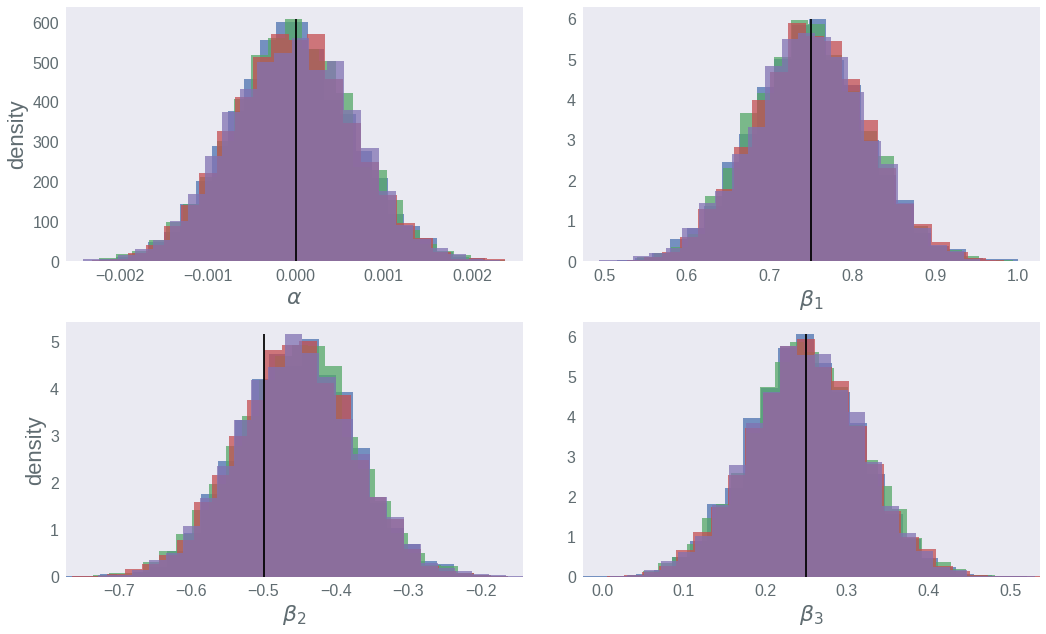
We can use the python interface to Stan, PyStan, to plot our realisations from the posterior. The histograms below show our posterior beliefs for \(\alpha\) and \(\beta_1\), \(\beta_2\) and \(\beta_3\). The true values are represented by the vertical black lines. See that in all the cases we are able to accurately recover the true parameter values from the data alone.
Posterior predictives in Stan
Posterior predictive
distributions represent
our beliefs about the distribution of new data, given the data which we have already
observed. We can use the generated quantities block in Stan to compute our posterior
predictive distributions during parameter inference:
data {
    // Order of AR process
    int<lower=0> P;
    // Numer of observations
    int<lower=0> N;
    // Observations
    vector[N] y;
}
parameters {
    // Additive constant
    real alpha;
    // Coefficients
    vector[P] beta;
    // Standard deviation of the noise
    real<lower=0> sigma;
}
transformed parameters {
    // Consider mu as a transform of the data, alpha and beta
    vector[N] mu;

    // Initial values
    mu[1:P] = y[1:P];

    for (t in (P + 1):N) {
        mu[t] = alpha;
        for (p in 1:P) {
            mu[t] += beta[p] * y[t-p];
        }
    }
}
model {
    // Increment the log-posterior
    y ~ normal(mu, sigma);
}
generated quantities {
    // Generate posterior predictives
    vector[N] y_pred;

    // First P points are known
    y_pred[1:P] = y[1:P];

    // Posterior predictive
    y_pred[(P + 1):N] = to_vector(normal_rng(mu[(P + 1):N], sigma));
}
The blue scatter markers in the plot below represent the simulated data: that which we observed. We then used our posterior beliefs about the parameter values to try and predict the simulated data, as if we’d never seen it before. We do so using the posterior predictive distribution.
The mean of our posterior predictive distribution is given by the red line. Although the posterior predictive mean makes for an informative point estimate, as Bayesians we are also interested in the uncertainty in our predictions.
The two shaded green areas represent 50% and 95% credibility intervals of our posterior predictive beliefs. That is, we predict with probability 0.5 that the next data point, given the previous \(p\) data points, will lie in the darker-green region. Similarily, we believe with probability 0.95 that the next observed data point, given the \(p\) observations before it, will be contained in the lighter-green region.
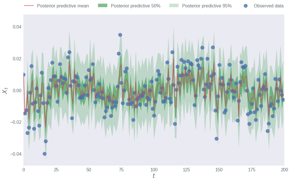
From this plot we can see that our model and parameter estimates can accurately capture and predict the simulated data. We see that about half of the observed points lie in the 50% credibility interval. As expected, we only observed about 5% of the observations (here, 4 points out of a total of 200) to lie outside the 95% credibility interval.
Posterior predictive distributions can provide a good way to assess the fit of a model to data. Of course, the practitioner would always be best advised to use a number of different metrics to assess model fit, and this represents only one such method.
Conclusion
Autoregressive models are popular models with many use cases. We saw how we can use Stan to fit such a model to real data. Having completed such a fitting, it is then important that the practitioner returns to assess how well the model fits the data. There are many different ways to assess model fit. One such method is to make use of a posterior predictive distribution. Stan code was provided to compute the posterior predictive distribution of an autoregressive model with order \(p\).