Plot publication-quality figures with matplotlib and LaTeX

22 Dec 2017

Figures are an incredibly important aspect of effectively communicating research and ideas. Bad figures are bad communicators: difficult to understand and interpret. They rear their ugly heads only to nauseate the reader and detract from the accompanying text. Good plots, however, are clear and concise. They seamlessly blend with their accompanied text and complement its narrative. Well executed figures should leave our readers informed, soothed, and certainly not nauseated.

So, if you care about your research (and since you’re here I’m going to take that as a given) you should care about your figure presentation too. Producing graphics isn’t the most exciting aspect of research (although I seem to have missed that memo), but it is an essential and unavoidable part of it.

This post will introduce the core-concepts you’ll need to produce publication-quality plots using the Python plotting package matplotlib and typesetting language LaTeX.

Seamless embedding in LaTeX

To ensure that our plots blend nicely into our LaTeX documents we need to avoid scaling our plots. When we scale our figures in LaTeX (typically with a \includegraphics[width=\textwidth] command), it isn’t just the graphical elements of our plots that are scaled: it’s also the text elements (axis labels, legends, titles, etc.). Scaling our graphics makes it difficult to control the font size and appearance in our finished plot.

To avoid scaling our graphics in LaTeX, we will use matplotlib to create our plots in the exact dimensions we wish them to be in our final document. With this the figure created in matplotlib will be the exact same figure that appears in our final document; no scaling, no surprises.

With scaling and text size taken care of, we can then instruct matplotlib to use LaTeX to typeset all the text elements in our plot. We can then match the font in our document body and plots. It’s only a minor alteration, but its this attention to detail which separates the good from the bad from the ugly.

Determining figure size

The key to seamlessly blending your matplotlib figures into your LaTeX document is in determining the desired dimensions of the figure before creation. In this way, when you insert your figure it will not need to be resized, and therefore font size and aspect ratio will be preserved.

Our first step to creating appropriately sized figures is to determine the textwidth of our LaTeX document. To do this we can make use of the \showthe command. Simply insert \showthe\textwidth into the preamble or main body of your .tex document.

% your document class here
\documentclass{report}
\begin{document}

% gives the width of the current document in pts
\showthe\textwidth

\end{document}

Recompile your .tex document. Compilation should be halted when the compiler hits the \showthe command, outputting the textwidth:

> 345.0pt.
l.5 \showthe\textwidth

Here we see that our document is 345pts wide. If compilation didn’t halt, you can find your document’s textwidth in its associated .log file (you’ll want to use a ctrl+f or grep here as the log file is rather verbose).

If you’re working with a document typeset in columns, you should use \showthe\columnwidth to determine the columnwidth of your document rather than its textwidth.

To specify the dimensions of a figure in matplotlib we use the figsize argument. However, the figsize argument takes inputs in inches and we have the width of our document in pts. To set the figure size we construct a function to convert from pts to inches and to determine an aesthetic figure height using the golden ratio:

def set_size(width, fraction=1):
    """Set figure dimensions to avoid scaling in LaTeX.

    Parameters
    ----------
    width: float
            Document textwidth or columnwidth in pts
    fraction: float, optional
            Fraction of the width which you wish the figure to occupy

    Returns
    -------
    fig_dim: tuple
            Dimensions of figure in inches
    """
    # Width of figure (in pts)
    fig_width_pt = width * fraction

    # Convert from pt to inches
    inches_per_pt = 1 / 72.27

    # Golden ratio to set aesthetic figure height
    # https://disq.us/p/2940ij3
    golden_ratio = (5**.5 - 1) / 2

    # Figure width in inches
    fig_width_in = fig_width_pt * inches_per_pt
    # Figure height in inches
    fig_height_in = fig_width_in * golden_ratio

    fig_dim = (fig_width_in, fig_height_in)

    return fig_dim

For convenience, you may wish to keep the set_size function in a module my_plot.py. Using this function we may create a figure which fits the width of our document perfectly:

import matplotlib.pyplot as plt
# if keeping the set_size function in my_plot module
from my_plot import set_size

width = 345
fig, ax = plt.subplots(1, 1, figsize=set_size(width))

If you desire to create a figure narrower than the full textwidth you may use the fraction argument. For example, to create a figure half the width of your document:

fig, ax = plt.subplots(1, 1, figsize=set_size(width, fraction=0.5))

Having plotted on and saved this figure instance, insert it into your .tex document with the graphicx package:

\begin{figure}
  \centering
  \includegraphics{figure_name.pdf}
\end{figure}

Note here the absence of scaling (there’s no [width=\textwidth] magic). In fact, now the figure size is set in matplotlib the width= argument of \includegraphics has become superfluous.

Figure size addendum

You may find it useful to predefine widths which you use regularly in your set_size function. Examples could be the textwidth of your thesis document, a journal you submit to, or a beamer template. Our amended function may include the lines:

    if width == 'thesis':
        width_pt = 426.79135
    elif width == 'beamer':
        width_pt = 307.28987
    else:
        width_pt = width
    # Width of figure
    fig_width_pt = width_pt * fraction

Handling multiple Axes

It’s often easier to handle subfigures at the matplotlib level, rather than within LaTeX. To produce plots made of multiple subplots we need to reconsider our set_size function.

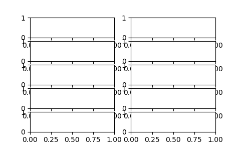
Consider a figure arranged into a grid with 5 rows and 2 columns of subfigures. Using our set_size function results in subfigures with unsightly aspect ratios:

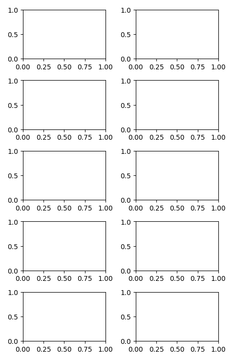
Fortunately, our function is easy to adapt. Simply add the default argument subplots=(1, 1) to the definition of set_size. Along with this, you must alter the line which calculates the figure height to fig_height_in = fig_width_in * golden_ratio * (subplots[0] / subplots[1]). With this, we would initialise a figure with 5 rows and 2 columns of Axes as fig, ax = plt.subplots(5, 2, figsize=set_size(width, subplots=(5, 2))):

With the above amendments, your set_size function should resemble something like:

def set_size(width, fraction=1, subplots=(1, 1)):
    """Set figure dimensions to avoid scaling in LaTeX.

    Parameters
    ----------
    width: float or string
            Document width in points, or string of predined document type
    fraction: float, optional
            Fraction of the width which you wish the figure to occupy
    subplots: array-like, optional
            The number of rows and columns of subplots.
    Returns
    -------
    fig_dim: tuple
            Dimensions of figure in inches
    """
    if width == 'thesis':
        width_pt = 426.79135
    elif width == 'beamer':
        width_pt = 307.28987
    else:
        width_pt = width

    # Width of figure (in pts)
    fig_width_pt = width_pt * fraction
    # Convert from pt to inches
    inches_per_pt = 1 / 72.27

    # Golden ratio to set aesthetic figure height
    # https://disq.us/p/2940ij3
    golden_ratio = (5**.5 - 1) / 2

    # Figure width in inches
    fig_width_in = fig_width_pt * inches_per_pt
    # Figure height in inches
    fig_height_in = fig_width_in * golden_ratio * (subplots[0] / subplots[1])

    return (fig_width_in, fig_height_in)

Text rendering with LaTeX

To really make our figures blend into our document we need the font to match between our figure and the body of our text. This topic is well-covered in matplotlib’s documentation, though I cover it here for completeness.

We shall use LaTeX to render the text in our figures by updating our rc settings. This update can be used to ensure that our document and figure use the same font sizes. The example below shows how to update rcParams to use LaTeX to render your text:

"""A simple example of creating a figure with text rendered in LaTeX."""

import numpy as np
import matplotlib.pyplot as plt
from my_plot import set_size

# Using seaborn's style
plt.style.use('seaborn')
width = 345

tex_fonts = {
    # Use LaTeX to write all text
    "text.usetex": True,
    "font.family": "serif",
    # Use 10pt font in plots, to match 10pt font in document
    "axes.labelsize": 10,
    "font.size": 10,
    # Make the legend/label fonts a little smaller
    "legend.fontsize": 8,
    "xtick.labelsize": 8,
    "ytick.labelsize": 8
}

plt.rcParams.update(tex_fonts)

x = np.linspace(0, 2*np.pi, 100)
# Initialise figure instance
fig, ax = plt.subplots(1, 1, figsize=set_size(width))
# Plot
ax.plot(x, np.sin(x))
ax.set_xlim(0, 2 * np.pi)
ax.set_xlabel(r'$\theta$')
ax.set_ylabel(r'$\sin (\theta)$')

Although this solution works just fine, it can become cumbersome to include this code to set fonts at the top of every one of your plotting routines. If you want to make things easier, it can be convenient to package your rc settings up into a style sheet. You can determine where matplotlib stores your style sheets with the following:

import os.path as path
import matplotlib as mpl
print("Your style sheets are located at: {}".format(path.join(mpl.__path__[0], 'mpl-data', 'stylelib')))

In the directory determined above you can create a new file tex.mplstyle with the following contents:

text.usetex: True
font.family: serif
axes.labelsize: 10
font.size: 10
legend.fontsize: 8
xtick.labelsize: 8
ytick.labelsize: 8

At the top of your plotting routines it is then sufficient to simply call plt.style.use('tex') to set all your text with LaTeX.

Colour and styling

One of the first things that a reader will notice about your figures is their colour scheme and styling. Many matplotlib users are living in the past with an old install of the package. More recent releases of matplotlib (>= v2.0) feature improved styling. This excellent talk from Scipy’s 2015 conference delves into some of the theory behind the new default colourmap. If you aren’t sure how to get the latest install, you can refer to the documentation provided by matplotlib.

Matplotlib provides many different style sheets for you to try out. You can list the available styles with

import matplotlib.pyplot as plt
plt.style.available

Style sheets allow the user to effortlessly swap between styles without having to alter their plotting routines. As an example, to change to the seaborn style we would use plt.style.use('seaborn'). Style sheets are additive, and it is possible to combine multiple styles. For example, to use seaborn’s styling with our LaTeX fonts (a personal favourite), we would do:

plt.style.use('seaborn')
plt.style.use('tex')

Save format

Not all file formats were created equal. If you are submitting figures to a journal you must first check which formats they will accept.

However, if the choice is up to you I would strongly recommend the use of a file format which can store vector images. Vector images allow the reader to zoom into a plot indefinitely, without encountering any pixelation. This is not true of raster images. Examples of raster image formats are .png and .jpeg; examples of vector graphic formats are .svg and .pdf. If, for whatever reason, you need to use a raster format - you’d be best advised to use .png and not .jpeg.

Below we create a simple figure and save it in the .pdf format. To remove excess whitespace which matplotlib pads plots with we may use bbox_inches='tight':

"""A simple example of creating a figure and saving as a pdf."""
import matplotlib.pyplot as plt
from my_plot import set_size
import numpy as np

# Using seaborn's style
plt.style.use('seaborn')
# With LaTex fonts
plt.style.use('tex')
width = 345

x = np.linspace(0, 2 * np.pi, 100)
# Initialise figure instance
fig, ax = plt.subplots(1, 1, figsize=set_size(width))

# Plot
ax.plot(x, np.sin(x))
ax.set_xlim(0, 2 * np.pi)
ax.set_xlabel(r'$\theta$')
ax.set_ylabel(r'$\sin (\theta)$')

# Save and remove excess whitespace
fig.savefig('example_1.pdf', format='pdf', bbox_inches='tight')

Summary

In this post we have seen how easy it is to change the style of our plots. We have learnt that to effectively present figures in a document we must take care to create a figure of the correct dimensions. With the correct dimensions our figure avoids any unwanted scaling and change in aspect ratio. After a brief discussion of why we should save our figures in the .pdf format, we discussed how to use LaTeX to render the fonts in our figures. Putting all these things together we can now produce truly publication-quality plots, and embed them in our work.